
Abstract
Herein I quantify the thermal effect of replacing the front door of my house. I acquired data with two temperature sensors I built using ESP32 microcontrollers and deployed inside and outside the house. Two weeks of temperature data were acquired both before and after the door replacement. The relative overnight cooling rates inside and outside the house, in the absence of artificial heat sources, are compared to Newton’s Law of Cooling, i.e. that the rate of indoor temperature decrease is proportional to the temperature difference between the inside and outside of the house. This basic analysis indicates that the cooling timescale of the house is about 24 hours and did increase with the replacement of the door, as expected, by about 30 minutes or 2%. However, this analysis also uncovers a more complex inside air temperature relaxation profile, presumably because inside air temperature is influenced both by conductive cooling from the house walls as well as from air leaking directly from the outside. In order to address this a model is constructed that dynamically couples the indoor and outdoor air temperatures with an (unmeasured) temperature of the walls of the house. Fitting this model to the data yields best-fit cooling constants for this system both before and after door replacement that acceptably capture the house cooling dynamics; both wall conduction and leaks of outside air. These fits to the house cooling system indicate that replacement of the door increased the cooling time constant of the house by as much as 10%: from 26 to 28 hours, also the impact of air leaks was substantially reduced. The data and analysis details for this blog post are in a github repository.
Data Collection
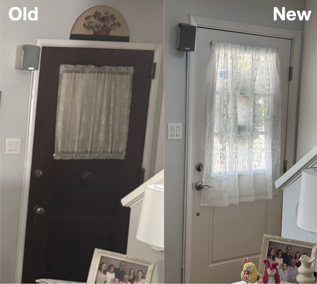
In anticipation of a long overdue replacement of the antique (estimated 1860’s) front door to my house with a modern, weatherproof model, I constructed a couple basic temperature sensors. To do this I used a couple of extra XIAO ESP32S3 microcontrollers that I had laying around. I’ve come to like the ESP-IDF development framework for programming the ESP32 family of chips. The code to program the ESP32S3 is here. The microcontroller interfaces with an MCP9808 temperature sensor over I2C and makes the data available by running a webserver on my WiFi network. It queries the temperature sensor every second with a read_temperature(¤t_temperature) call. The webserver can receive two URI requests; one for the temperature and another for WiFi radio connection signal strength. Each device runs a mDNS service that allows it to be found on my network with the name temp-sensor-1 or temp-sensor-2 respectively. I then run a python script temperature_logger.py on a computer that queries and logs the temperature from each device.
| Temperature sensors |
|---|
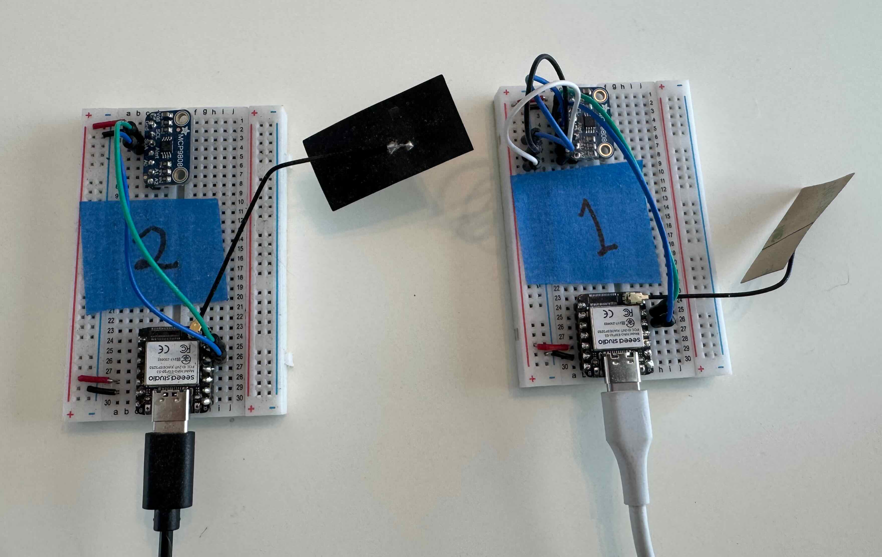 |
| My identical pair of remote temperature sensors. Each is based on a XIAO ESP32S3 microcontroller that polls the MCP9808 temperature sensor via an I2C interface and runs a web server connected to my WiFi network to which it posts the data. The rectangular WiFi antenna sticks out to the right of each ESP32 board. |
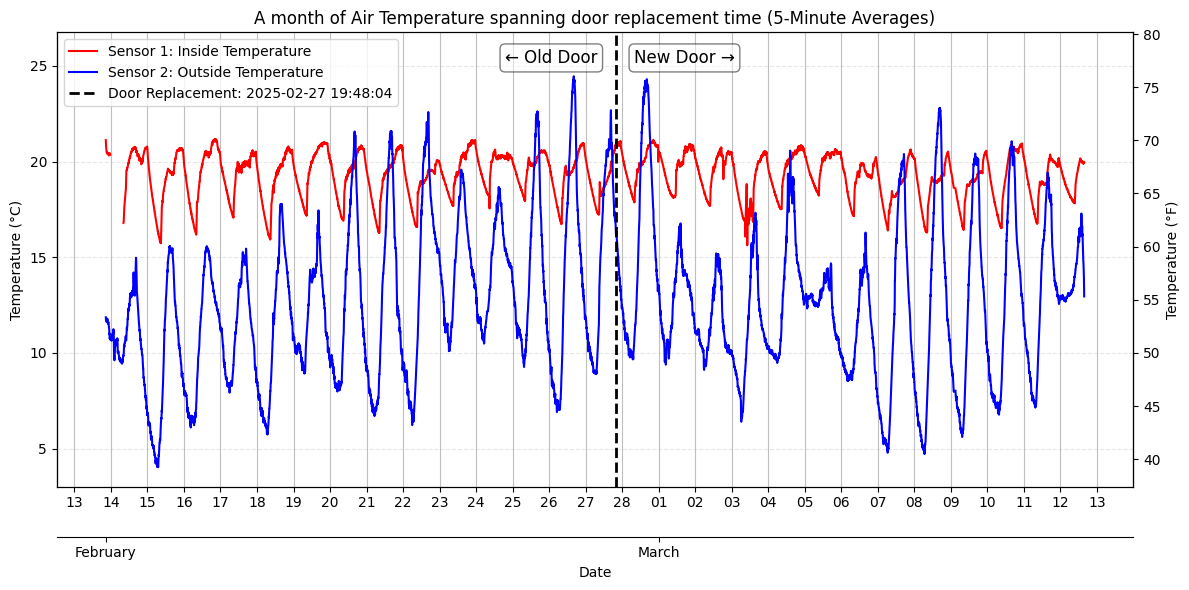
I collected roughly two weeks of data both before and after the door replacement. All internal heating (i.e. the furnace) was turned off each night so the house was allowed to naturally cool overnight from roughly the same initial temperature (~ 70° Fahrenheit). Plotting the raw indoor and outdoor temperatures over the entire duration (below) shows the diurnal oscillation period of the outdoor temperature (blue) as well as the nightly cooling curve (starting around midnight, signified by the vertical date line) of the inside temperature (red), however, beyond that, this data doesn’t yield any obvious trends to my eye. More analysis will need to be employed to see if there are underlying trends.
Data Analysis
Newton’s Law of Cooling
The initial goal of this study is to model the nighttime cooling profiles with Newton’s Law of Cooling. Specifically, I assume that the rate of change of the house’s inside temperature, $T_i$, is proportional to the difference between the outside and inside temperatures, $T_o - T_i$:
\[\begin{equation} \frac{dT_i}{dt} = K(T_o - T_i) \end{equation}\]which is simply to say that the colder it is outside, the faster the house will cool off. The goal is to determine the cooling constant, $K$, both before and and after door replacement to see if it is different. In theory $K$ will be smaller after the door is replaced, meaning the house will cool more slowly for a given temperature difference $T_o - T_i$.
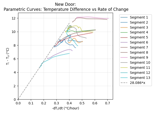
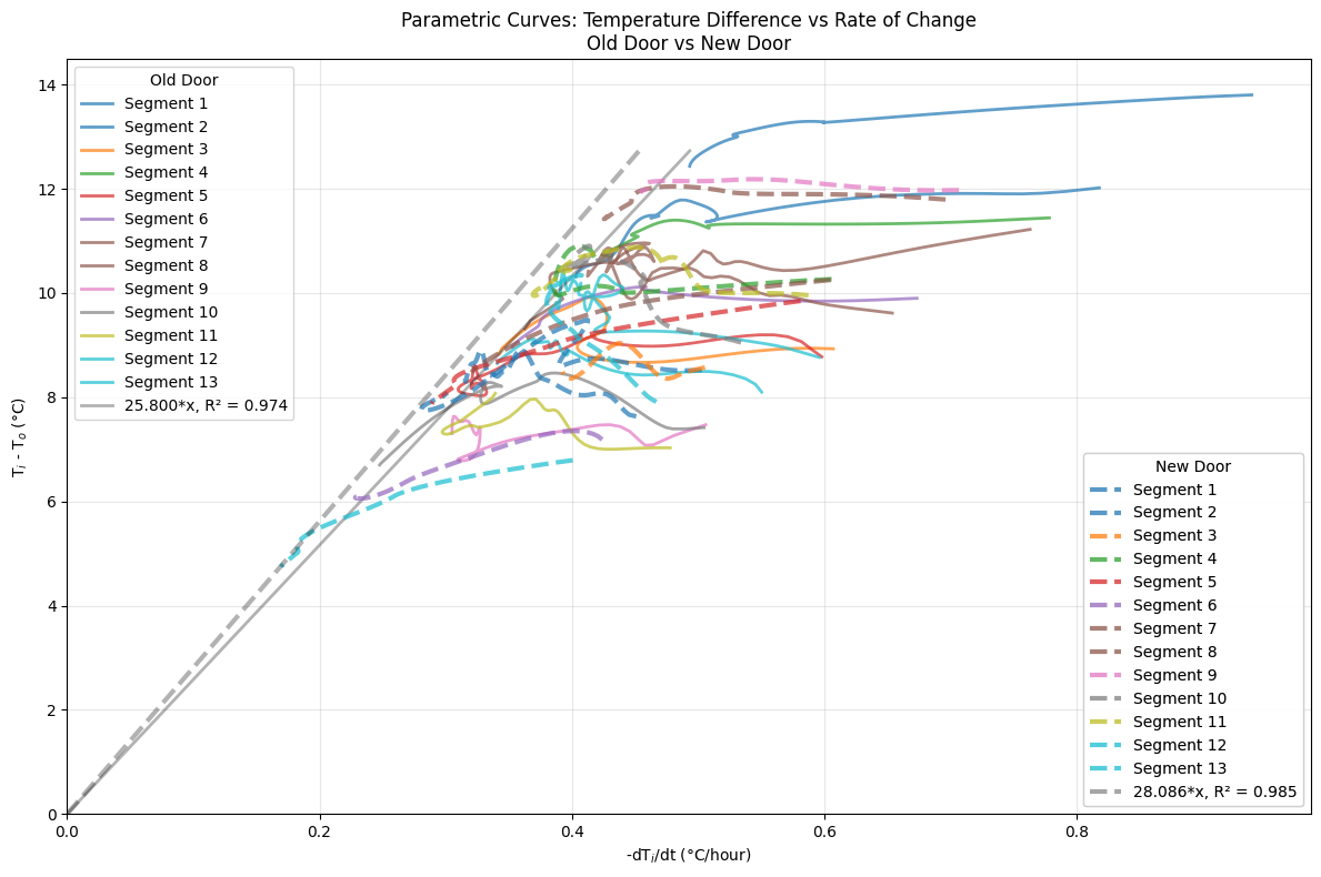
The temperature history is filtered to select the nightly segments of time for which the furnace is off and the house cools naturally. This nightly cooling data is shown in the figures below. Note that there is typically a period of relatively rapid cooling, ~1°C/hour, for roughly an hour at the beginning of the evening, when the heat is first turned off. This is presumably due to cold outside air leaking into a porous house and replacing a portion of the warm, inside air (we will address this with the dynamical model). Also, in the morning, after sunrise (but before the denizens have turned on the furnace) there is often a rapid decline in the cooling rate as well as the temperature difference between the inside and outside, as the outdoors begin to warm. (Note that the time of sunrise is calculated for each day for my location in Livermore, CA.) Both of these epochs present more complex dynamics than the simple cooling law we are interested in modeling, so we discard them both for our fits. These appropriately filtered nightly cooling segments can now be parametrically plotted with the inside temperature cooling rate versus the temperature difference between the inside and outside, shown below. This is the correlation we wish to fit to Newton’s Law of Cooling and the respective fits for the Old and New door are plotted. This gives the initial result that for the Old Door, $1/K = 23.6$ hours and for the new door, $1/K = 24.2$ hours. As such it appears that the replacement of the door has increased the cooling timescale of the house by a bit over a half an hour, or about 2%, which is encouraging! Interestingly, the residuals of these fits show an anticorrelation: the cooling rate tends to slowly decrease throughout the night faster than the difference between inside and outside temperatures would predict. So there appears to be some cooling behavior beyond what is predicted by a simple application of Newton’s Law of Cooling.
| Temperature Difference vs Inside Cooling Rate | |
|---|---|
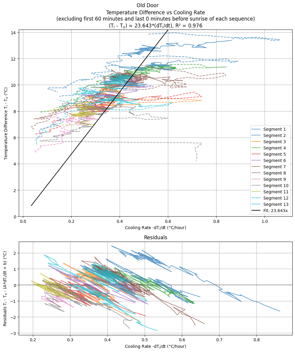
|
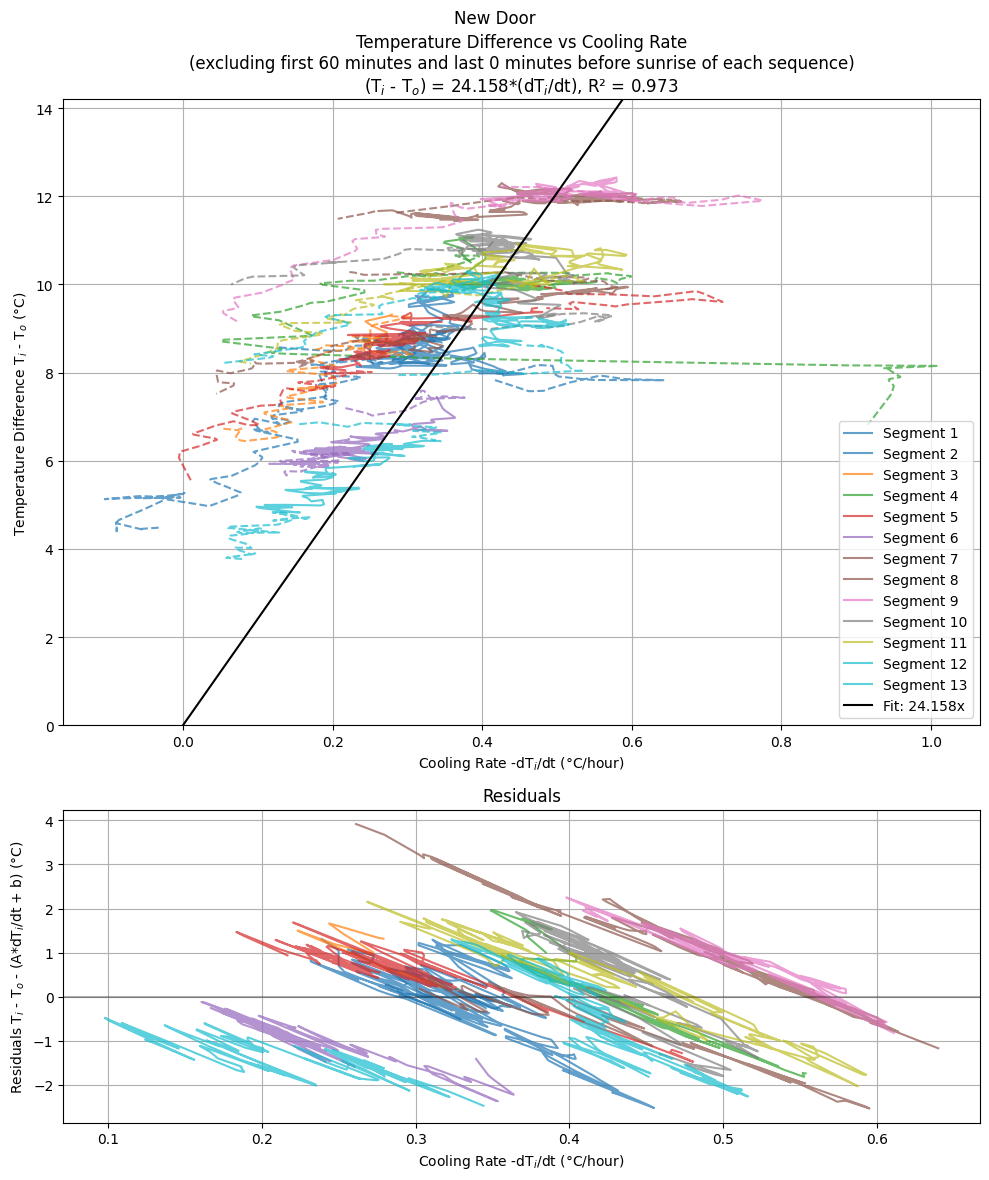
|
| Parametric plots of each night's cooling segments with the Old (left) and New (right) doors. The best fit for Newton's Law of Cooling is shown for each. Data (dashed lines) at the beginning of each evening's cooling curve and after sunrise is excluded from the fit (see text for details). Note a systematic anticorrelation in the residual plots: the cooling rate decreases more slowly than the temperature difference over the course of the evening. | |
There is some uncertainty in the fit of the cooling constant depending how much of the early rapid-cooling phase to include, how much data before or after sunsrise should be included and since the cooling rate, $dT_{i}/dt$, is a derivative which can be noisy, the amount of smoothing applied with make a difference. For that reason I model the data over an ensemble of variations of these parameters, specifically:
- initial time to skip: 60 to 80 minutes
- end time relative to sunrise: -30 to 30 minutes
- derivative resampling window: 5 to 10 minutes
An ensemble of 200 fits are constructed for both the old and new door data, randomly varying these paramters.
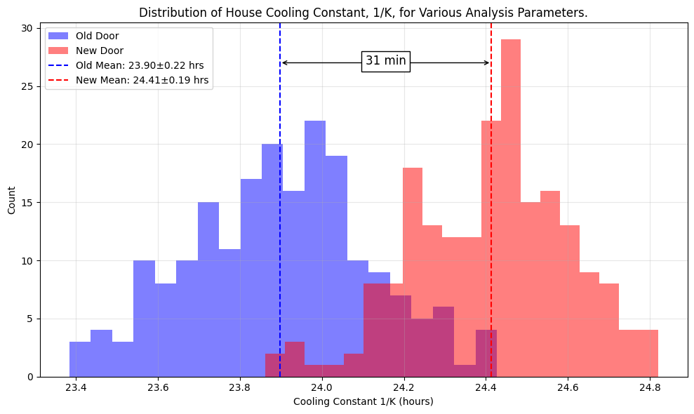
|
|
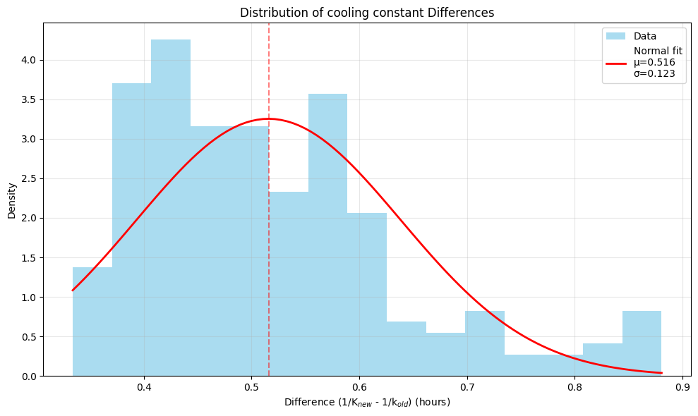
|
| The distribution of fits of the cooling constant for both the Old and New door gives a distribution that is significantly longer for the Old door than for the New door (Left figure). Plotting the difference between these cooling curves (Right figure) gives a mean difference of roughly 0.52 ± 0.12 hours (31 ± 7 minutes). Note that, although I'm calculating a standard deviation, this distribution has a p-value of 0.0 and so is not normal. This suggests that replacement of the old door has increased the 24 hour cooling time by roughly a half hour, or 2%. This is a small, but non-negligible increase. | |
Time Dependent Cooling
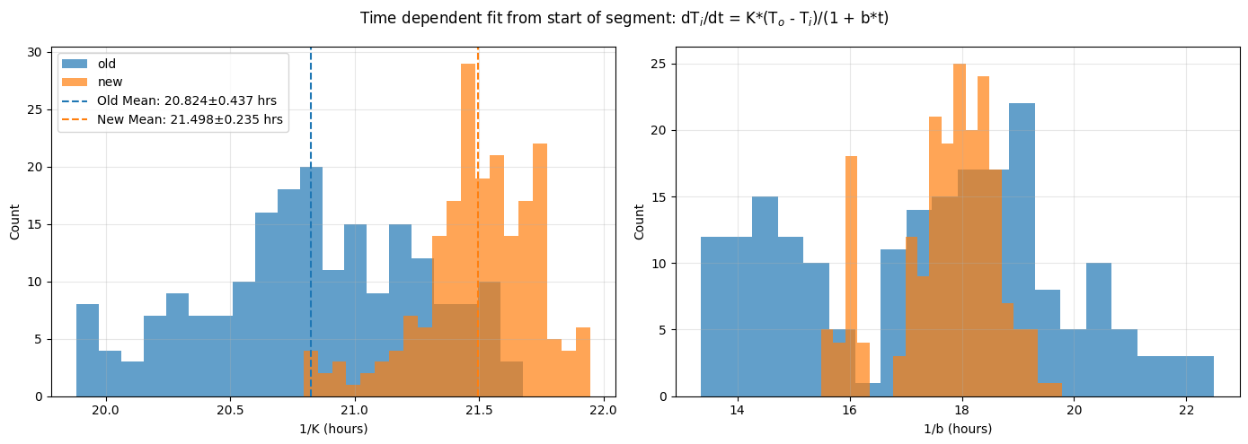
As previously mentioned, Newton’s Cooling Law doesn’t fully explain the data. On a given night, the rate of cooling tends to decrease a little faster than the decrease in the temperature difference between the inside and outside as can be seen from the cooling segments data. So we can attempt to fit a more elaborate cooling law with a time dependence to the cooling rate
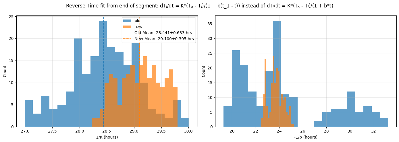
\[\begin{equation} \frac{dT_i}{dt} = \frac{K}{1 + b \tau} (T_o - T_i) \end{equation}\]where $\tau$ is the time within the cooling segment. We fit this function from the beginning of each cooling segment, i.e. $\tau = t$, and also from the end of the segment, i.e. $\tau = t\_1 - t$ where $t\_1$ is the last time in the segment. As with the previous time independent cooling law fit, an ensemble of 200 fits of this function are performed, varying the segment start and end time and resampling window. The resulting histograms are plotted below. A key observation is that when fitting this temporally decaying function from the start of the segment (so $K$ is representative of the decay constant at the beginnings of the segments) the decay constant is shorter, $1/K \approx 21$ hours, than the constant-time fit above; $1/K \approx 24$ hours. Also, when fitting from the end of the segment, when the cooling rate tends to be lowest, the decay constant is significantly longer; $1/K \approx 29$ hours.
The key take-away is that the observation of the longer decay constant in New door as compared to the Old door persists in these data. Fitting the cooling time decay from the beginning of the segments gives $1/K$ of 20.8 and 21.5 hours for the Old and New doors respectively, and measuring from the end of the pulse gives 28.4 and 29.1 hours. This is consistent with the previous result that the cooling timescale of the house was increased by roughly 30 minutes by replacing the Old door.
The cooling rate time decay constant, $b$, doesn’t exhibit an offset between the Old and New door, which isn’t surprising. It is interesting that the spread in the values of $1/b$ is noticably narrower for the New door than for the Old door. One might hypothesize that this is due to the reduction in the Old door’s drafty leaks which can cause rapid cooling, particularly early in an evening’s cooling cycle. Applying a dynamical cooling model in the next section might shed some light on this.
|
|
|
|
| Time-dependent cooling constants. The key take-away is that the cooling timescale 1/K for these fits shows the same difference between the Old and New door as observed in the time independent fit; the New door's cooling constant is roughly 30 minutes longer than that of the Old door. | |
Solving a More Complete Dynamical Cooling Model
Upon consideration, it appears that a more elaborate process is at play. The indoor air temperature has relatively little heat capacity compared to the house or the great outdoors and so is significantly influenced both by being in contact with the walls of the house as well as by leakage of air from the outdoors. Unfortunately, we don’t directly measure the wall temperature, but we can model the dynamical cooling of both the walls of the house as well as the indoor air temperatures as they interact with the outdoor temperature. So we define a model where air and walls of the house are driven by their interactions with their counterparts
\[\begin{align} \text{(indoor air cooling rate)} &= \text{(warming by the walls)} + \text{(leakage from outdoor air)} \\ \text{(wall cooling rate)} &= \text{(cooling by outdoor air)} + \text{(cooling by indoor air)} \end{align}\]which can be written more precisely as
\[\begin{align} \frac{dT_i}{dt} &= K_1(T_w - T_i) + K_2(T_o - T_i) \\ \frac{dT_w}{dt} &= K_3(T_o - T_w) + K_4(T_i - T_w) \ \ . \end{align}\]The walls of the house will have signficant heat capacity and thus their temperature, $T_w$, will change the most slowly. The indoor air temperature, $T_i$, has relatively small heat capacity and will react strongly to contact with the walls and leakage of outside air. Our goal is to indirectly infer the cooling of the wall as well as the mixing of leaked outside air solely from the observations of the inside air temperature.
The model is as follows: when the furnace it turned off at night it is assumed that the walls of the house and the air inside are at the same temperature, i.e. $T_w(t=0) = T_i(t=0)$. The inside air temperature, with its relatively small heat capacity, will cool faster than the wall due to cool outside air leaking into the house via the $K_2$ term. This relatively rapid cool down of the inside air due to leakage will eventually be offset by the now warmer walls heating the air via the $K_1$ term. The walls of the house, with their large heat capacity, will cool slowly by contact with the outside via the $K_3$ term, which is the dominant term of the system. Since the heat capacity of the inside air is much, much smaller than that of the house, we can safely neglect the inside air heating the walls, so we set
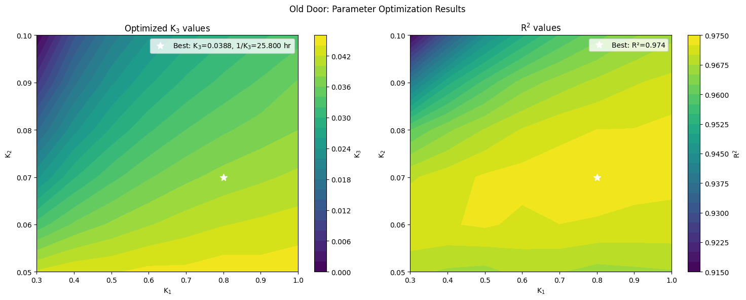
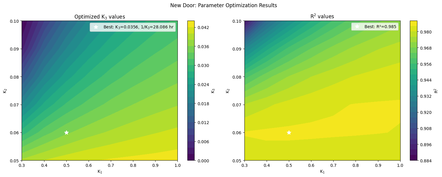
\[K_4 = 0 \ \ .\]As such we have a three-parameter model for the cooling of the inside air, $T_i$, and house walls, $T_w$, in the presence of a measured outdoor temperature, $T_o(t)$. Since we have also measured the inside air, $T_i(t)$, we can fit the solution, $T_{i,\text{sol}}(t)$, of this set of ODEs to the measured $T_i(t)$ and find the parameters $K_1$, $K_2$, $K_3$ that give the best match via a least-squares minimization: $\text{min}((T_{i,\text{sol}}(t) - T_i(t))^2)$. Performing this optimization for both the Old Door and New Door data will provide information about how the cooling model of the house has changed due to the door replacement.
|
|
|
|
| Optimization of the K1, K2, and K3 parameters demonstrated here by rastering through a grid of possible values for K1, K2. At each of these points the optimal solution for K3 is iteratively found to maximize the coefficient of determination, R2. As such we get some idea of the shape of the solution manifold. All K constants have units of 1/hour. | |
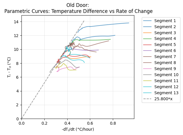
| Dynamical Simulations of Temperature Difference vs Inside Cooling Rate | |
|---|---|
|
|
| Similar to the parametric cooling figure above, but instead of data, here are the solutions to the dynamical model for each evening's cooling segment. The dashed line shows the 1/K3 slope. This illustrates how K3, that governs how fast the house walls cool due to the outside air, acts as an asymptotic limit to the cooling rate. This is in contrast to the parameter K used to fit the mean cooling effect seen in the data, which is why the 1/K line goes thru the center of the data. | |
The resulting best-fit solutions are:
| Parameter [1/hour (hour)] | Description | Old Door | New Door |
|---|---|---|---|
| K₁ (1/K₁) | warming of inside air by house walls | 0.8 (1.25 hours) | 0.5 (2 hours) |
| K₂ (1/K₂) | leakage of outside air to the inside | 0.07 (14.3 hours) | 0.06 (16.6 hours) |
| K₃ (1/K₃) | cooling of the house walls by outside air | 0.0388 (25.8 hours) | 0.0356 (28.1 hours) |
|
| For reference, the dynamical cooling solutions for both the Old and New Doors along with their respective 1/K3 parameter fits. This highlights how subtle the difference between the Old (1/K3 = 25.8 hours) and New (1/K3 = 28.1 hours) Door solutions is. |
It is a heartening result that we were able to find solutions of this dynamical system that are consistent with the hypothesized interaction of inside and outside air with the walls of the house. The plots of these solutions on top of the data (below) show generally good agreement. As such the obtained values of the cooling constants $K_1$, $K_2$, $K_3$ should give some insight into the cooling dynamics. A key point to note from the parameter optimization results is that the optima for both the Old and New door are relatively broad, with a wide region of values with coefficients of determination, $R^2$, near 1.0. As such, we will only interpret these results qualitatively. However, again, this analysis suggests a general locus of parameters that reasonably fit the data.
All three parameters, $K_1$, $K_2$, $K_3$ indicate weaker coupling after the New Door was installed (i.e. the inverse of each is a longer cooling timescale). As such, rather than specifying a particular cooling process having been altered by the door replacement, the fits suggest that all such cooling processes were reduced. One wouldn’t expect that $K_1$, the rate at which the house walls warm the inside air, to change much with the replacement of the door, for instance, however the best fit parameters changed by almost a factor of 2. However, we note that the parameter optimization plots show a relatively flat (i.e. weak) sensitivity to $K_1$, so one could hypothesize a fixed value $K_1$ both before and after door replacement and test how that affects the solution of the other parameters. Such elaborations in analysis would deserve a larger, more systematically careful dataset than the one acquired for this study, and so we forgo further such analysis here.
Summary
We have satisfactorily acheived the goal of measuring and quantifying the cooling rate of my house both before and after the replacement of an antique Old Door with a New modern one. The empirical result that the cooling timescale from Newton’s Law for the inside air temperature of the house is about 24 hours and increased by about 30 minutes with the replacement of the door appears to be robust, both when considering a simple, constant cooling rate and when a time dependent rate is employed to capture the extraneous cooling behavior. Further, we hypothesized a dynamical model of both the inside and outside air interacting with the solid walls of the house as a way to explain the more complex cooling evolution seen in the data. This model qualitatively captures the cooling rate of the inside air – both the early, rapid cooling presumably due to outside air leaking in, as well as the gradual decrease in this cooling rate throughout the night. To pursue this line of study further one would want to gather more data, including measurements of the wall temperature, to more rigorously test this model.
Reference
- temperature_sensor_esp32_mcp9808 - Repository of data and analysis for this notebook
Figure Appendix
Cooling Data Segments
| Night-time Cooling Data Segments | |
|---|---|
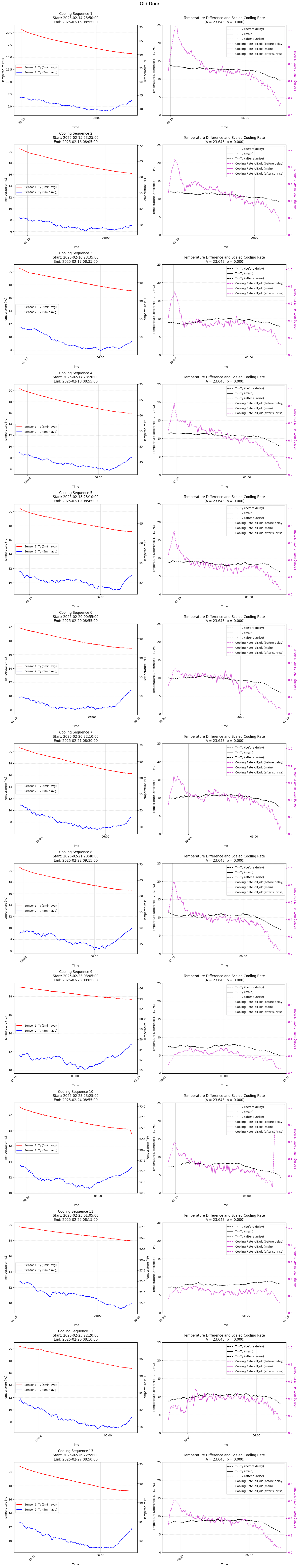
|
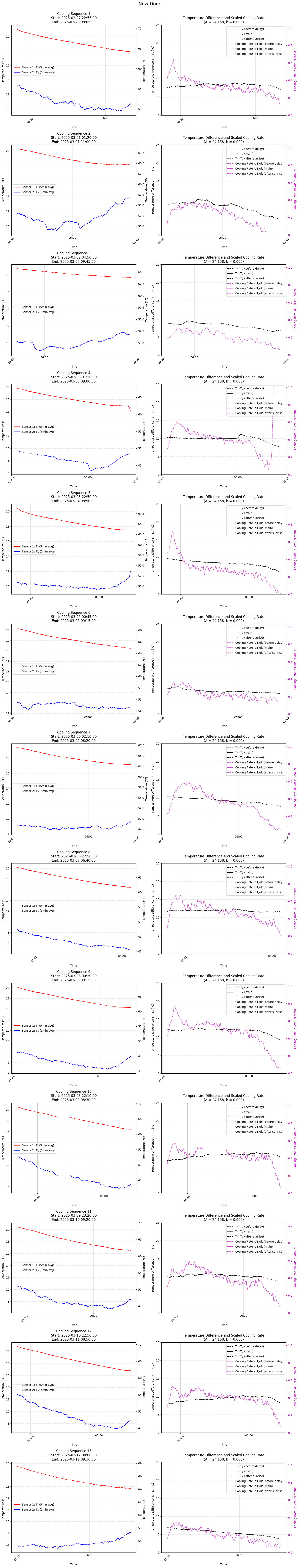
|
| Comparison of cooling data before (left) and after (right) door replacement. The left plot of each pair is simply the raw temperature data from each sensor. On the right plot of each pair, the data excluded from the fit is dashed; specifically the first 60 minutes of cooling and data after (date specific) sunrise. The cooling (magenta) and temperature difference (black) curves are scaled by the fit to give intuition for how good it is. A careful eye will notice that the cooling rate (magenta) tends to decrease slightly faster than the temperature difference (black) over the course of the night. This motivates the time dependent fit. | |
Cooling Data Segments with Cooling Solutions
| Night-time Cooling Data Segments with Cooling Solutions | |
|---|---|
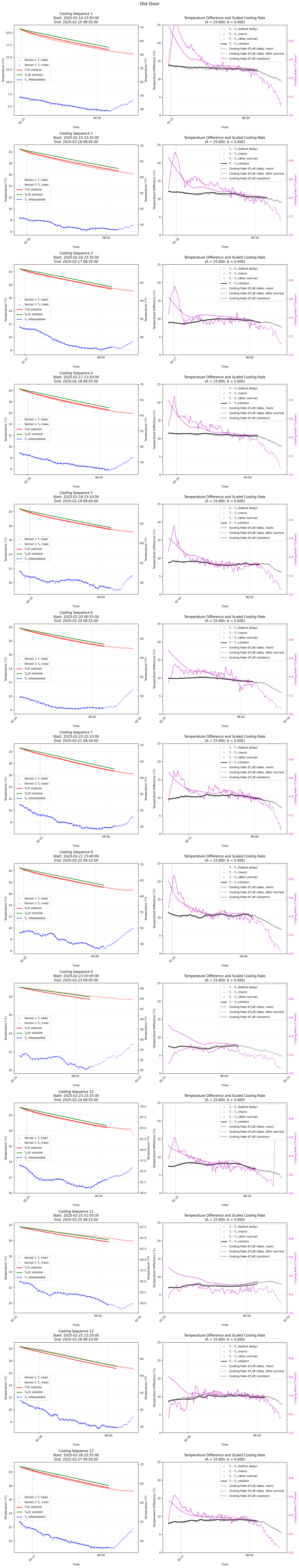
|
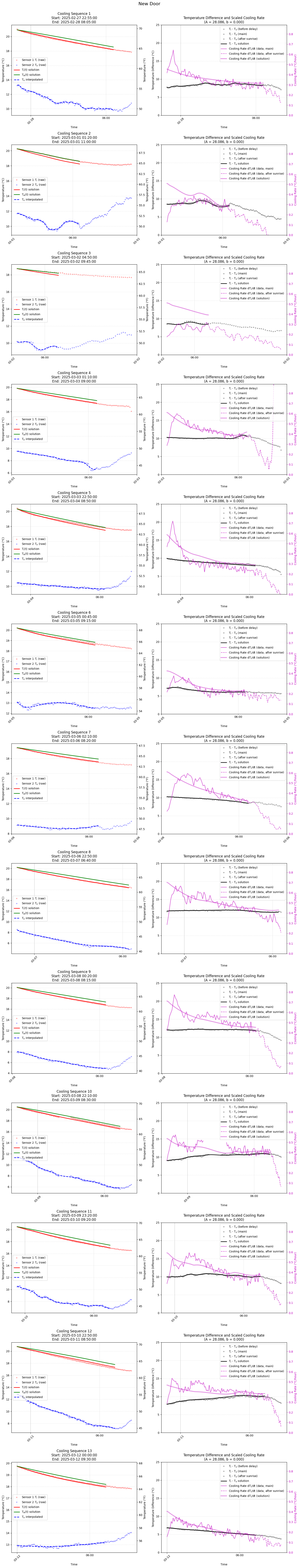
|
| Similar to the the cooling data figures above except that the best-fit dynamical cooling solution is also plotted as solid curves. In particular, on the left of the pair of plots the solutions for the inside air (red) and house wall (green) temperatures are shown, and on the right of the pair of plots the inside air cooling rate solution is plotted. (Note that the house wall temperature (green) was not explicitly measured, so only the inferred solution is shown.) Also note that (magenta) cooling rate data on the right plots is including the first 60 minutes of data (unlike the plots above), but not that after sunrise, since this dynamical fit is attempting to capture the early cooling behavior (presumably due to air leaks). The outside temperature (blue on left plots) is measured and is an input to the dynamical solution. | |